Text-As-Treatment
Text-As-Treatment is a key setting where gpi_pack is especially useful. Instead of directly modeling texts, we use the internal representations of LLMs to estimate treatment effects. This approach improves accuracy and computational efficiency. In this section, we provide an overview of the Text-As-Treatment setting and demonstrate how to use gpi_pack to estimate treatment effects with the internal representations of LLMs.
Note
This part is based on our paper Causal Representation Learning with Generative Artificial Intelligence: Application to Texts as Treatments. Please refer to the paper for the technical details.
What is Text-As-Treatment?
Text-As-Treatment refers to scenarios where participants receive various texts, and the goal is to determine how one specific feature of the texts (e.g., topics or sentiments) influences downstream outcomes. A primary challenge in this setting is that texts inherently contain other features that might confound the relationship between the feature of interest and the outcome.
To address this challenge, our paper proposes using LLMs’ internal representations to bypass the direct modeling of texts. We introduce a representation learning method called deconfounder, which enables us to estimate the treatment effects of the feature of interest without directly observing all confounding features. The deconfounder is estimated using TarNet, which takes the internal representations as input and predicts outcomes under both treatment and control conditions using a shared deconfounder. The following figure illustrates the architecture of TarNet:
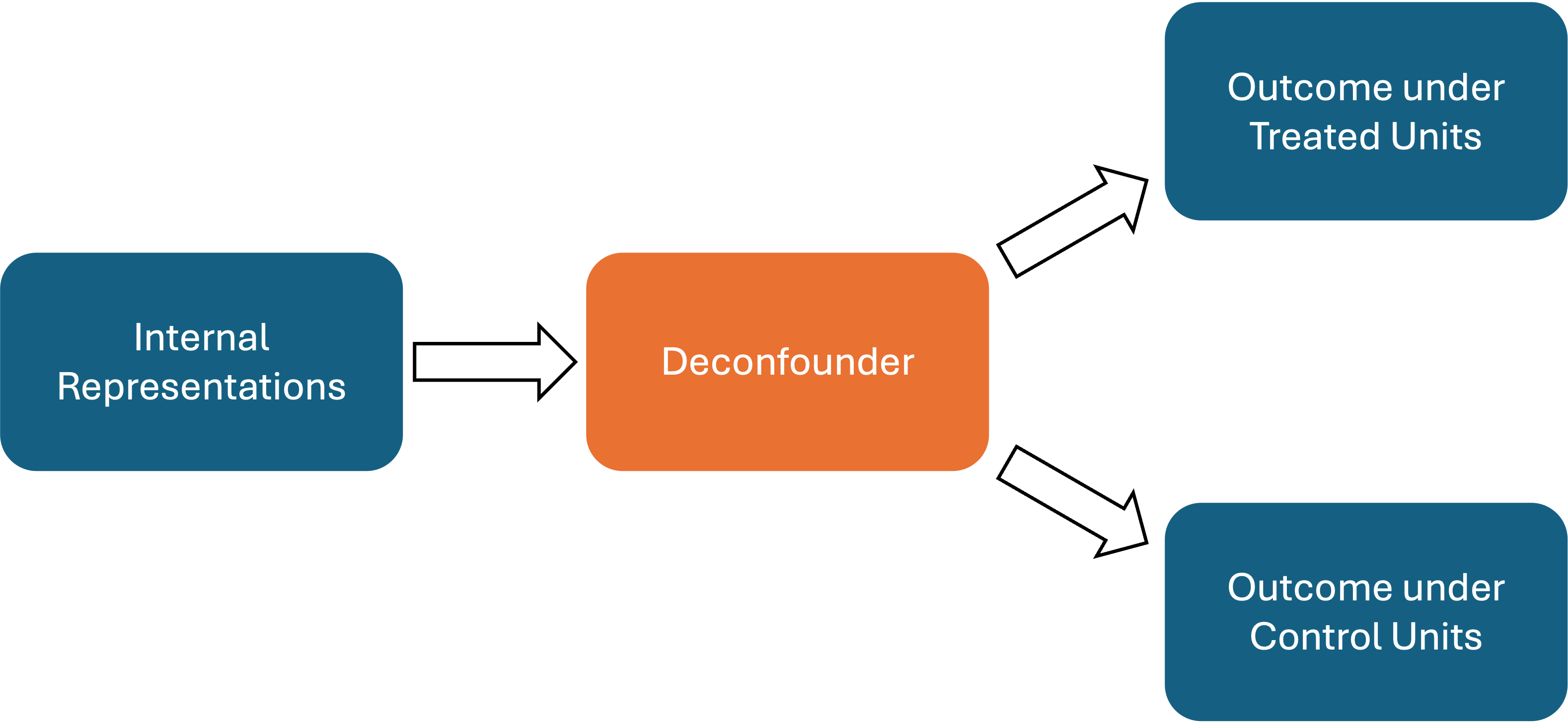
Once the deconfounder and the outcome models are estimated, a propensity score model is built based on the deconfounder. Finally, the estimated outcome models and propensity score model are used together with double machine learning techniques to estimate treatment effects.
How to estimate treatment effects
gpi_pack offers the wrapper function estimate_k_ate to streamline the estimation of treatment effects using LLMs’ internal representations. This function handles all the necessary steps, including deconfounder estimation and propensity score estimation, so you only need to provide the data.
Suppose you have a DataFrame df containing the treatment variable, outcome variable, and texts, and you have already extracted the internal representations of the LLMs (saved as .pt files). Below is an example demonstrating how to use estimate_k_ate .
# loading required packages
import pandas as pd

# create a data frame
df = pd.DataFrame({
    'TreatmentVar': [1, 0, 1, 0, 1],
    'OutcomeVar': [1, 0, 1, 0, 1],
    'Text': [
        'Create a biography of an American politician named Nathaniel C. Gilchrist',
        'Create a biography of an American politician named John Doe',
        'Create a biography of an American politician named Jane Smith',
        'Create a biography of an American politician named Mary Johnson',
        'Create a biography of an American politician named Robert Brown',
    ]
})
Step 1: Load the Internal Representations
First, load the internal representations using the load_hiddens function:
# loading required packages
from gpi_pack.TarNet import estimate_k_ate, load_hiddens

# load hidden states stored as .pt files
hidden_dir = <YOUR-DIRECTORY> # directory containing hidden states (e.g., "hidden_last_1.pt" for text indexed 1)

hidden_states = load_hiddens(
    directory = hidden_dir,
    hidden_list= df.index.tolist(), # list of indices for hidden states
    prefix = "hidden_last_", # prefix of hidden states (e.g., "hidden_last_" for "hidden_last_1.pt")
)
Note
If you have not extracted internal representation, please refer to the section Generating Texts with LLaMa3.
Step 2: Estimate the Treatment Effects
Once the internal representations are loaded, use estimate_k_ate to estimate the treatment effects:
# estimate treatment effects
ate, se = estimate_k_ate(
    # Data (Inputs)
    R= hidden_states,
    Y= df['OutcomeVar'].values,
    T= df['TreatmentVar'].values,

    # Hyperparameters (optional)
    K=2, #K-fold cross-fitting
    lr = 2e-5, #learning rate
    architecture_y = [200, 1], #outcome model architecture
    architecture_z = [2048], #deconfounder architecture
)
To compute a 95% confidence interval for the treatment effect estimate, use the following code:
# calculate 95% confidence interval
lower_bound = ate - 1.96 * se
upper_bound = ate + 1.96 * se

print(f"ATE: {ate}, SE: {se}, 95% CI: ({lower_bound}, {upper_bound})")
# ATE: 0.5, SE: 0.1, 95% CI: (0.3, 0.7)
How to control confounders
In some cases, you may want to control for confounders that are not included in the texts. gpi_pack supports this via the estimate_k_ate function in two ways:
Method 1: Using a Formula with a DataFrame
If your DataFrame includes confounders as columns, specify a formula (e.g., formula_c = "conf1 + conf2") along with the DataFrame in the function call:
# Method 1: supply covariates with a formula and DataFrame
ate, se = estimate_k_ate(
    R= hidden_states,
    Y= df['OutcomeVar'].values,
    T= df['TreatmentVar'].values,
    formula_c="conf1 + conf2",
    data=df,
    K=2, #K-fold cross-fitting
    lr = 2e-5, #learning rate
    #Outcome model architecture
    # [100, 1] means that the deconfounder is passed to the intermediate layer with size 100,
    # and then it passes to the output layer with size 1.

    #Outcome model architecture
    # [100, 1] means that the deconfounder is passed to the intermediate layer with size 100,
    # and then it passes to the output layer with size 1.
    architecture_y = [200, 1],

    #Deconfounder model architecture:
    # [2048] means that the input (hidden states) is passed to the intermediate layer with size 2048.
    # The size of last layer (last number in the list) corresponds to the dimension of the deconfounder.
    architecture_z = [2048],
)
Method 2: Using a Design Matrix
Alternatively, create a design matrix of confounders and pass it to the C argument:
Note
The design matrix should be a NumPy array or a list of values.
# Method 2: supply covariates using a design matrix
import numpy as np #load numpy module
C_mat = np.column_stack([df['conf1'].values, df['conf2'].values])

ate, se = estimate_k_ate(
    R= hidden_states,
    Y= df['OutcomeVar'].values,
    T= df['TreatmentVar'].values,
    C=C_mat, #design matrix of confounding variable
    K=2, #K-fold cross-fitting
    lr = 2e-5, #learning rate

    #Outcome model architecture
    # [100, 1] means that the deconfounder is passed to the intermediate layer with size 100,
    # and then it passes to the output layer with size 1.
    architecture_y = [200, 1],

    #Deconfounder model architecture:
    # [2048] means that the input (hidden states) is passed to the intermediate layer with size 2048.
    # The size of last layer (last number in the list) corresponds to the dimension of the deconfounder.
    architecture_z = [2048],
)
Visualizing Propensity Scores
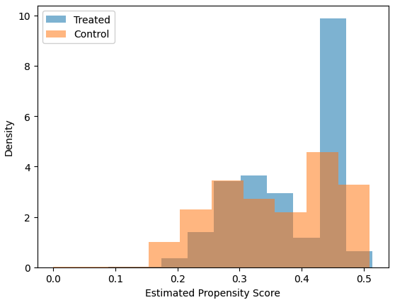
For the Text-As-Treatment setting, it is crucial to assume that the textual feature and the confounding features are disentangled—a property known as separability. Visualizing the propensity scores can help diagnose whether this assumption holds. If the propensity scores are extreme (close to 0 or 1), it may indicate that confounding features are entangled with the treatment feature of interest.
By default, the estimate_k_ate function allows you to visualize the propensity scores by setting plot_propensity=True. Below is an example:
# estimate treatment effects
ate, se = estimate_k_ate(
    R= hidden_states,
    Y= df['OutcomeVar'].values,
    T= df['TreatmentVar'].values,
    K=2, #K-fold cross-fitting
    lr = 2e-5, #learning rate
    architecture_y = [200, 1], #outcome model architecture
    architecture_z = [2048], #deconfounder architecture
    plot_propensity = True, #visualize propensity scores
)
Hyperparameters
The estimate_k_ate function accepts the following parameters:
R: list or np.ndarrayA list or NumPy array of hidden states extracted from LLM. Shape: (N, d_R) where N is the number of samples and d_R is the dimension of hidden states. You can load the stored hidden states using load_hiddens function.
Y: list or np.ndarrayA list or NumPy array of outcomes, shape: (N,).
T: list or np.ndarrayA list or NumPy array of treatments, shape: (N,). Typically binary (0 or 1).
C: list or np.ndarray, optionalA matrix of additional confounders, shape: (N, d_C). If provided, these will be concatenated to R along axis=1. You can pass either this parameter directly or use formula_c and data.
formula_c: str, optionalA Patsy-style formula (e.g., “conf1 + conf2”) that specifies how to build the confounder matrix from a DataFrame. If this is provided, data must also be provided, and C will be constructed via dmatrix(formula_c, data). Intercept is removed from the design matrix.
data: pandas.DataFrame, optionalThe DataFrame containing the columns used in formula_c. If formula_c is set, this parameter is required. The resulting design matrix is then concatenated to R as additional confounders.
K: int, default=2Number of cross-fitting folds (K-fold split).
valid_perc: float, default=0.2Proportion of the training set to use for validation when fitting TarNet in each fold.
plot_propensity: bool, default=TrueWhether to plot the propensity score distribution in the console or a graphing interface (implementation-specific).
ps_model: object, optionalA model/classifier used to estimate the propensity score. By default, we use a neural network with Spectral Normalization (to ensure Lipshitz continuity).
ps_model_params: dict, optionalHyperparameters for ps_model. For example, {“input_dim”: 2048} if using a custom model requiring an input dimension.
batch_size: int, default=32Batch size for TarNet training.
nepoch: int, default=200Number of epochs to train TarNet.
step_size: int, optionalStep size for the learning rate scheduler (if applicable).
lr: float, default=2e-5Learning rate for TarNet.
dropout: float, default=0.2Dropout rate for TarNet layers.
architecture_y: list, default=[200, 1]List specifying the layer sizes for the outcome heads (treatment-specific networks or final layers). For example, [200, 1] means that the outcome model has two hidden layers, the first with 200 units and the second with 1 unit.
architecture_z: list, default=[2048]List specifying the layer sizes for the deconfounder. For example, [2048, 2048] means that the deconfounder has two hidden layers, each with 2048 units.
trim: list, default=[0.01, 0.99]Trimming bounds for the propensity score. Propensity scores outside this range will be replaced with the nearest bound.
bn: bool, default=FalseWhether to apply batch normalization in TarNet.
patience: int, default=5Patience for early stopping in TarNet training (number of epochs without improvement).
min_delta: float, default=0Minimum improvement threshold for early stopping.
model_dir: str, optionalDirectory path where the model checkpoints might be saved. If provided, the best model will be saved here and loaded for predictions.
verbose: bool, default=TrueWhether to print additional information during training.