Customizing Your Analysis

While gpi_pack offers the wrapper function estimate_k_ate for the complete static GPI workflow, you may want to inspect or customize its individual stages. The procedure has three main steps:

Fit TarNet to learn a deconfounder and the outcome regression.
Estimate the propensity score from the held-out deconfounder.
Combine the nuisance estimates with the doubly robust score.

The examples below show the current lower-level APIs. They illustrate one outer held-out split; a complete cross-fitted analysis must repeat the procedure over all outer folds. Use estimate_k_ate when you do not need to customize those folds.

TarNet

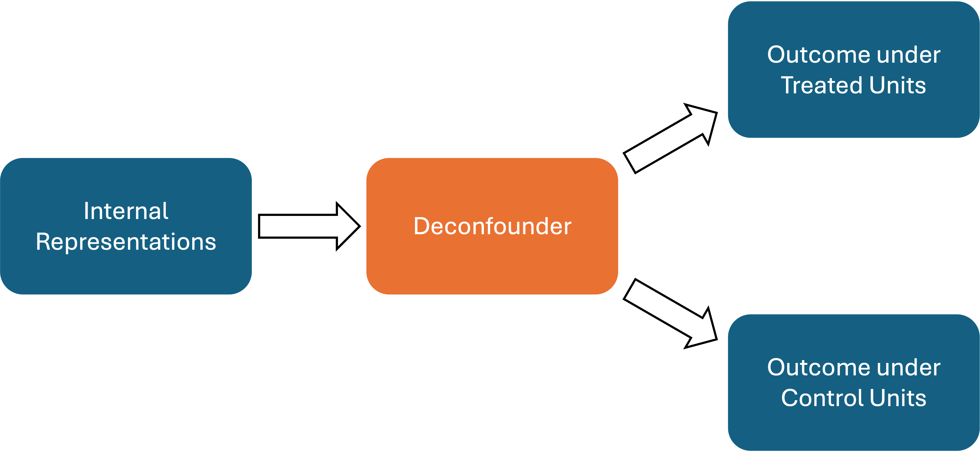
TarNet learns a shared representation from the generative-model features. It concatenates a supplied treatment value to that representation and passes the result through one treatment-conditioned outcome network. Consequently, call predict once with treatment zero and once with treatment one to estimate both potential outcomes.

import numpy as np
from sklearn.model_selection import train_test_split
from gpi_pack import TarNet

# Create one outer training/held-out split for illustration.
R_train, R_test, Y_train, Y_test, T_train, T_test = train_test_split(
    hidden_states,
    Y,
    T,
    test_size=0.5,
    random_state=42,
    stratify=T,
)

model = TarNet(
    epochs=100,
    batch_size=32,
    learning_rate=1e-3,
    architecture_y=[200, 1],
    architecture_z=[512],
    dropout=0.1,
    verbose=False,
)

best_validation_loss = model.fit(
    R=R_train,
    Y=Y_train,
    T=T_train,
    valid_perc=0.2,
    plot_loss=False,
)

y0_pred, deconfounder = model.predict(
    r=R_test,
    t=np.zeros_like(T_test),
)
y1_pred, _ = model.predict(
    r=R_test,
    t=np.ones_like(T_test),
)

predict returns PyTorch tensors. The deconfounder has width architecture_z[-1] when no additional covariates are supplied. If covariates are passed as C to fit, pass the corresponding held-out values as lowercase c to predict; they are appended to the returned deconfounder. For all arguments and return values, see TarNet.

Propensity Score Model

The propensity score is the probability of treatment conditional on the estimated deconfounder. gpi_pack provides SpectralNormClassifier, a feed-forward classifier whose linear layers use spectral normalization. Its constructor uses nepoch and lr rather than the TarNet names epochs and learning_rate.

from gpi_pack import SpectralNormClassifier

deconfounder_np = deconfounder.detach().cpu().numpy()

ps_model = SpectralNormClassifier(
    input_dim=deconfounder_np.shape[1],
    hidden_sizes=[128, 64],
    nepoch=100,
    batch_size=32,
    lr=1e-3,
    dropout=0.1,
)
ps_model.fit(deconfounder_np, T_test)

# Column 1 is Pr(T=1 | deconfounder).
ps_pred = ps_model.predict_proba(deconfounder_np)[:, 1]

The direct fit above demonstrates the classifier API only. It trains and predicts on the same observations, so these probabilities should not be used as the nuisance estimates in a causal analysis. predict returns hard class labels; use predict_proba(... )[:, 1] for binary propensity scores. See SpectralNormClassifier for the full classifier reference.

Cross-Fitted Score Contributions

estimate_psi_split performs the required inner cross-fitting of the propensity model. It divides the outer held-out observations into two halves, trains the propensity model on one half, predicts the other half, and then reverses the roles. When using the default classifier directly, supply its required input_dim through ps_model_params.

import numpy as np
from gpi_pack import estimate_psi_split

psi, ps_pred = estimate_psi_split(
    fr=deconfounder,
    t=T_test,
    y=Y_test,
    y0=y0_pred,
    y1=y1_pred,
    ps_model_params={"input_dim": deconfounder.shape[1]},
    trim=[0.01, 0.99],
    plot_propensity=True,
)

ate_for_this_outer_fold = np.mean(psi)
se_for_this_outer_fold = np.std(psi) / np.sqrt(len(psi))

The returned propensity scores follow the input row order. The returned psi values are concatenated in inner held-out-fold order, which does not affect their mean or standard deviation but does matter if you need to join scores back to individual rows. See estimate_psi_split for details.

Complete Cross-Fitting

The code above produces score contributions for only one outer held-out split. For a complete analysis, repeat the TarNet fit and the inner propensity cross-fit for every outer fold, then combine all score contributions. The wrapper estimate_k_ate implements this complete process and should be preferred unless the custom workflow preserves the same sample separation.